Method & Design
User Shelter
The main design of this work is to identify where a user took shelter at various times during Hurricane Sandy. From these points of interest, a Twitterers’s movement pattern during the hurricane can be analyzed to determine protective decisions they may (or may not) have made about their shelters.
Step 1. Identify Spatial Clusters

The DBScan algorithm is used here for density based clustering. Tweets are clustered by geospatial density. Benefits of this method include:
- Not necessary to define #clusters before hand (Like k-means).
- Includes a non-cluster group which can be thrown out.
Zero Confidence
The tweets that are unable to placed in a cluster are treated as noise. There are two attributes set from this cluster:
@unclassifiable = true (If there are no other clusters)
@unclassified_percentage = (number of tweets in non-cluster group) / (total tweets)
If unclassifiable, then that user is ignored for further analysis. The unclassified_percentage can be used as measure of confidence later in the analysis. if the majority of a user’s tweets land in the unclassifiable cluster, then it is hard to be sure that the clusters that were identified are accurate representations of the user’s potential shelter locations.
Step 3. Identify Temporal Spread
We must determine a user’s repetitive tweeting behavior to get the best idea of when and where they tweet. Empirical analysis and speaking with lead Geo-HCI researcher, Brent Hecht, shows that people generally seem to show repetitive tweet behavior at a given location. For example, watching television at home at night.
Dividing a 24 hour day into 8 separate time bins of 3 hours, the goal is to find repetitive temporal behavior.
Example:
Imagine two clusters of tweets: X and O:
| Hour | Day 1 | Day 2 | Day 3 | Day 4 | Day 5 | Day 6 | Day 7 | Day 8 | Day 9 |
|---|---|---|---|---|---|---|---|---|---|
| 1 | X | X | X | X | X | X | X | X | X |
| 2 | |||||||||
| 3 | O | ||||||||
| 4 | O | O | |||||||
| 5 | O | O | O | ||||||
| 6 | O | O | |||||||
| 7 | O | ||||||||
| 8 |
In this 9 day window, Each cluster of tweets had exactly 9 tweets, once per day. However, the temporal spread of the X tweets is only 1, meaning that each day the user tweeted from within the same 3 hour window.
The O tweets, however, have a temporal spread of 5, meaning that the 9 tweets in this cluster occurred sporadically over 21 hours of the day, each day.
Each cluster then gets a normalized t_score, which represents the temporal spread. Here is an extreme example for a particular user:
Cluster: 0  has 967 tweets with T_Score of 8.555335374493764e-06
Cluster: 4  has 56  tweets with T_Score of 0.00031887755102040814
Cluster: 3  has 49  tweets with T_Score of 0.001665972511453561
Cluster: 8  has 20  tweets with T_Score of 0.0025
Cluster: 2  has 15  tweets with T_Score of 0.0044444444444444444
Cluster: 11 has 9   tweets with T_Score of 0.012345679012345678
Cluster: 9  has 9   tweets with T_Score of 0.012345679012345678
Cluster: 7  has 6   tweets with T_Score of 0.027777777777777776
Cluster: 5  has 4   tweets with T_Score of 0.0625
Cluster: 1  has 4   tweets with T_Score of 0.0625
Cluster: 10 has 3   tweets with T_Score of 0.1111111111111111
Cluster: 6  has 3   tweets with T_Score of 0.1111111111111111
Cluster 0 is the obvious choice for a home location in this example and clusters 3 and 4 are very interesting as well. In the event a user tweeted from multiple clusters in a day, the cluster with the lowest t_score will be favored as the dominant location for that day. In searching for an evacuation, finding multiple days during the storm where this user did not tweet from location 0 would be a high indicator.
Before & After Home (Shelter) Locations
A user’s before_home shelter location is determined by the most tweeted from location with the lowest t_score before October 28 (the day before landfall). Similarly, the after_home location is determined by the most tweeted from location after November 8.
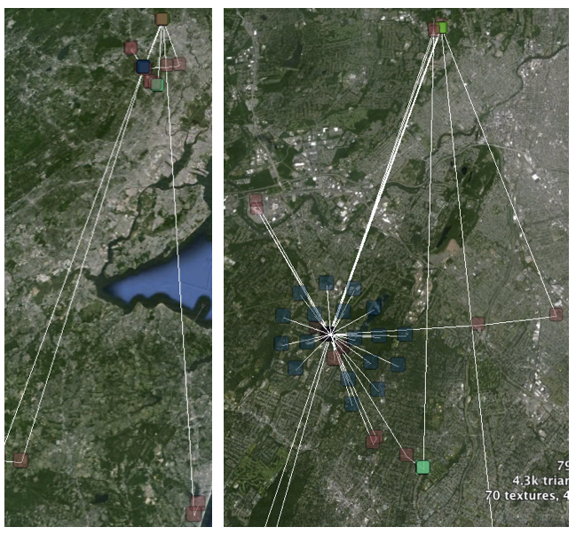
Here are a user’s before home & their most likely during the storm shelter location: